Nested Learning: Intuition Behind the Math (Part-I)

1. Introduction

Google Research recently released a groundbreaking paper that, in my opinion, is nothing short of a masterpiece. In this work, my aim is to simplify the concepts and mathematics provided in the paper and make it much more intuitive for a wider audience, while also providing my own insights and additions regarding the concept.

Before we delve into the world of Nested Learning, we must first familiarize ourselves with a few terms from the world of cognitive neuroscience. The way I have defined these terms may not be 100% biologically accurate, but represents the best approach to understanding them so as to make a meaningful connection with the intuition behind the development of the NL paradigm. Throughout this work, I will refer to “Nested Learning” as NL to save on some extra keystrokes.

2. Foundational Concepts from Cognitive Neuroscience

To understand the Nested Learning paradigm, we must first establish a conceptual bridge between neuroscience and machine learning. The following definitions are tailored to facilitate this understanding.

2.1 Memory

Think of memory as a physical configuration of wires inside your brain, analogous to wires inside any electrical appliance. These biological wires are what we refer to as synapses, and the term “memory” denotes a particular arrangement in which these synapses are attached and connected to each other inside your brain.

2.2 Associative Memory

Associative memory is the kind of memory that we as humans possess. It associates keys to their values. Consider it as a mathematical function like $y = 2x + 3$. For the value $x = 1$, we know that $y = 5$. This means the function maps $1 \rightarrow 5$. That is precisely what an associative memory does.

The difference is that in real life, the key or value fed to the function is not a number but a stimulus. For instance, when you read English text, your eyes perceive the shapes of letters and how they are written. These visual inputs are fed to your brain, which, as we just discussed, is an associative memory that maps these shapes to values. When you see the shape “A”, your brain immediately produces as output the sound “A”, and not just the sound—the output need not be just one value. It can be anything: this is a character from the English language, it is the first alphabet, etc. Whatever you have acquired as memory throughout your life via learning can be given as output.

Now, suppose I present you with a Cyrillic character. To you, it might not make any sense because you have no memory of it via learning. Therefore, the synapses of your brain have not wired themselves throughout your lifetime to map the meaning of this symbol to what it truly represents. But to a Russian speaker, this would immediately make sense—they would map it to the corresponding Cyrillic letter representing a particular sound, because their brain has the memory for it and their synapses are wired to map it correctly.

I hope this provides you with an understanding of associative memory (AM), as this is the most important concept you must grasp to understand the core of NL.

2.3 Learning

As stated in the original paper, people often use memorization and learning interchangeably, but learning is actually a subset of memorization. In other words, the act of acquiring meaningful memories is learning.

To clarify, suppose you are cooking Butter Chicken. First, you try to make it yourself and end up with “Burned God-knows-what Chicken.” Later, you watch a YouTube video and, following that video, you make the most delicious Butter Chicken. In both cases, you formed memories—your brain rewired itself. However, in the second case, you learned the correct method for making the chicken (this is learning), while in the first case, you learned what not to do to avoid burning the chicken again (also learning). But the memories from the first experience about how to cook, though stored in your brain, do not constitute effective learning in the positive sense.

2.4 Neuroplasticity

As you acquire more memory, the synapses inside your brain rearrange their connections to accommodate the new memory you have acquired, so that in the future when you encounter the same stimulus, your brain can map it correctly to whatever you have learned. In simple terms, the wires inside your brain change their physical connection patterns so that new outputs can be mapped.

3. Machine Learning Models as Associative Memories

Now let us transition to the world of Machine Learning and Deep Learning. If you are reading this work, I assume you have at least some understanding of what ML and DL mean and how they work. If not, I would suggest reviewing some textbooks before proceeding. However, you do not need extremely advanced knowledge, at least not initially. In the later sections, this might become more technical, particularly if you are unfamiliar with the Transformer architecture, but we will address that when necessary.

3.1 Models as Mathematical Functions

All Machine Learning models, whether they be Deep Learning architectures like MLPs and RNNs or even simple regressors like Linear Regression, are at their core mathematical functions. This is what we have been taught, and it is completely correct. As we discussed earlier, associative memory is also like a mathematical function. Therefore, you can think of all Machine Learning models as being associative memories.

All ML models are mathematical functions at their core. They take as input numbers—which can be a single number or an entire vector—and produce as output, again, numbers. In other words, they simply map inputs to outputs.

Now, what will be the output for a given input? That is the billion-dollar question, and we all know the answer: it depends on the weights (or parameters) of the model.

For example, $y = 2x + 5$ and $y = 3x + 7$ will both give different outputs for the same input $x = 1$ because the weights $[2, 5]$ in the first equation are different from $[3, 7]$ in the second one.

3.2 The First Analogy: Weights as Synapses

This is where we draw our first analogy. Think (or better yet, imagine and visualize) these weights as a particular configuration of wires (or synapses) inside the model’s brain. Different weights represent different ways in which the synapses are connected to each other and to different nodes inside the model’s brain, such that the flow of data is different, and therefore for the same input, the output is different.

We know that when an ML model learns, it is trying to find the optimal set of parameters (weights and biases) that minimize the loss function (its objective). There is nothing wrong with this definition. It is simply that Nested Learning attempts to change the perspective on how you view the phenomenon of model learning and training.

3.3 Model Training as Neuroplasticity

We can say that as the model learns new weights by minimizing the loss function, it is simply rewiring its synaptic connections to accommodate the input-output mapping of the data point it just observed. We can treat all inputs to any model (or memory, as we shall call it) as an experience, and the process of learning—known in humans as neuroplasticity—is exactly how we can conceptualize model training as well. The changing of model weights is equivalent to someone updating the wiring of the synapses inside the model’s brain.

You might be wondering why we are delving deep into this perspective, as the standard mathematical approach has been sufficient so far for understanding what is happening and gaining intuition. Why this extra analogy? This might seem trivial at this point, but the analogy is key to maintaining grasp of what is happening in NL once we dive deeper into multi-layered memory systems. At that stage, if you attempt to analyze everything purely mathematically, it becomes too complex, and you might find it difficult to have that intuitive feeling of “Yes, I understood that.”

4. Optimizers as Memory and Wirer

This is one of the key areas where the paper makes a huge leap in terms of perspective. The idea of viewing models as memories and weights as synapses is neither novel nor revolutionary, as it is quite evident to anyone who has given some thought to this connection. The field of Deep Learning, in general, owes heavily to neuroscience.

However, treating optimizers as yet another deeper layer of memory is something truly new, which opens doors to creating far more expressive and sophisticated deep learning models.

4.1 Optimizers as Wirers

The job of a wirer, as the name suggests, is to update the synaptic connections or, in our case, update the weights of the brain. This role is fulfilled by optimization equations, as these equations are what update the weights.

The simplest wirer we all know is standard gradient descent and all its variants (stochastic, batch, etc.):

This represents a single-layered memory model, where the memory is the main model, represented by its weights $W$, and the wirer is gradient descent (e.g., SGD).

When you train any model—whether it be a vanilla MLP or even a basic linear regressor—using raw gradient descent, you are making a single layer of memory learn from experiences, where the experiences are nothing but the data points. The wirer simply observes how well the model’s experience was based on an objective (we will discuss this in detail later) and, using only the current experience (data point), changes the wiring. Since the SGD equation takes into account the gradient from the loss output given by only the present data point or batch, this leads to a specific behavior.

This is why using only GD or SGD produces noisy changes: the wirer is changing the connections by looking at only the present batch. It is trying to create a wire combination pattern that will satisfy all data points seen so far, but it forgets what the previous data points were. All it does is change the weights and hope that the new changes do not adversely affect the output for previous data points. While trying to satisfy the requirements of new points, it might inadvertently disturb the requirements of old ones, as it has no memory of the old requirements in the first place.

4.2 Optimizers as Memory

The biggest problem with the naive wirer described above is that it has no memory. It is merely a simple agent whose only job is to, based on current data point requirements and performance on the objective, update the wire configuration (weights). But what if we gave it access to memory as well? That is exactly what momentum does.

We all use momentum; in fact, hardly anyone today uses raw GD or SGD. The equations for momentum-based gradient descent are:

Think of momentum as another “memory” in itself. The only difference is that it does not have weights, so it has no synaptic connections. All it remembers is a weighted average of the requirements (gradients of loss) from all past data points. We can conceptualize it as just a single box that stores a single value, not a complicated brain-like memory with wiring that can map inputs to outputs.

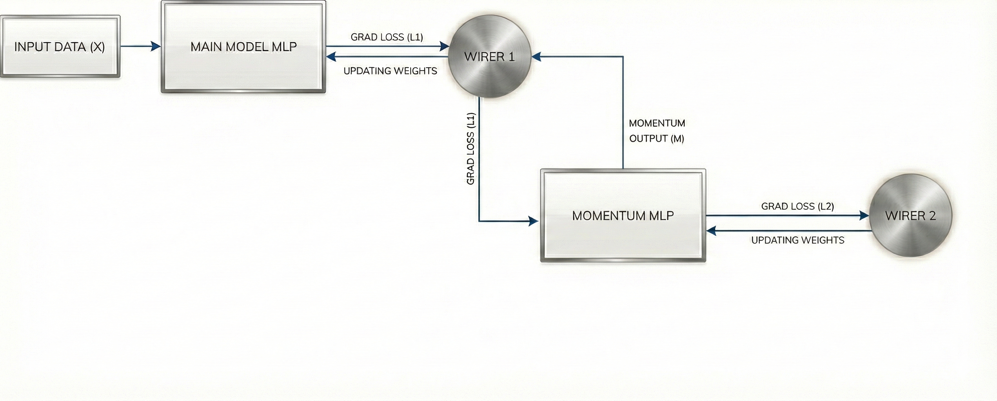
A very important point here is that since we have now defined momentum as its own “memory,” albeit a simple one, someone needs to open the box and update the stored value for it as well. We call this agent Wirer No. 2. Even though its job is much simpler, it is still updating the memory just like Wirer No. 1 does for the main model.

Now Wirer No. 1 has access to the stored value of the momentum memory, which represents the requirements (based on gradients of losses) of all past data points, not just the current one. Therefore, it is much more careful and takes into account the needs of all past points before rewiring, making the learning process for the main model much smoother.

So, we have:

• Wirer 1: $W_{t+1} = W_t + M_{t+1}$
• Wirer 2: $M_{t+1} = \beta M_t - \eta \nabla_W L$

Remember how I mentioned earlier that the wirers are nothing but the equations themselves that update the synapses. You can clearly see above that both wirers are equations that update the two memories $W$ and $M$.

Before I conclude this section, I want to reiterate that momentum ($M$) and the main model ($W$) are both memories. However, at this point in time, they are different kinds of memories. The main model is an “associative memory” similar to how our brains work—with a complicated network of synapses represented by its weights, which maps inputs to outputs. In contrast, momentum is a simple storage box that merely stores a value. In this case, it stores a running weighted average of all past gradients of the loss function across all batches.

In the next section, we will modify momentum from being a simple box-like memory that just stores values to also being an associative memory with its own set of weights (synaptic connections), thereby enabling it to map inputs to outputs.

5. Optimizers as Associative Memories

The original condensed version of the paper becomes quite abstract and concise at this point, so this is where my originality comes in—interpreting what they said and providing my own ideas.

The paper suggests three different ways in which momentum could be improved:

1. Use a pre-conditioner $P$ and train momentum to map input gradients to this $P$ more effectively. This $P$ could be anything useful, such as the Hessian.
2. Improve the objective function such that the update equation—how the wirer connects the synapses or stores the value in the box—becomes more effective.
3. Give momentum a better memory by making it an MLP.

All these ideas could be combined, in my opinion, to create a very strong framework that can then be further nested.

5.1 Making Momentum an MLP

We need to make our optimizer memories smarter and better. As a first step toward this goal, the paper suggests giving momentum its own set of weights, making it an MLP in itself.

The reasoning is straightforward. By passing the gradient through an MLP, $M$ can now extract much deeper semantics and transform the gradient using its weights in complex ways. The output could potentially hold more topographical information, such as Hessian information, which would help Wirer No. 1 make better choices about how to rewire (update $W$) for improved mapping.

The output of the MLP can be the vector $P$, which, as we stated, could encompass a wide variety of information useful for navigating the loss landscape. Therefore, the momentum would now, as an MLP, learn to compress (or map) the input gradient $\nabla L$ to the output $P$.

Now, for any complex associative memory to function, we know it must learn. It learns by getting rewired. But how it gets rewired depends upon how well it performed on the objective given to it.

5.2 Objective Functions

When a model is trained, its weights are updated based on how it performed on its objective. For instance, in linear regression, the objective is to minimize the function:

Think of this as a checklist of requirements given by the wirer, which the brain “checks off” based on the data point experience it just received. The fewer requirements it satisfied, the greater the adjustment needed, and thus the greater the change. The crux is that how much the wirer will change, and how it will change the synaptic connections (weights), depends upon the performance on the objective.

5.3 Objectives for Momentum

Momentum is now an MLP, so it needs an objective. Without one, how will Wirer No. 2 assess its requirements and make changes to the synapses?

The paper proposes two kinds of objectives that the momentum wirer can use to evaluate the M-brain. Here, we will discuss the one deemed more effective: an L2 regression-like loss function.

This means we want our momentum MLP output to be as close to $P$ as possible. Therefore, Wirer No. 2 now receives an upgrade in form. Since it is an equation:

• Wirer 2: $M_{t+1} = \alpha M_t - \eta \nabla_M L^{(2)} (M_t (\nabla L^{(1)}))$
• Wirer 1: $W_{t+1} = W_t + M_{t+1} (\nabla L^{(1)})$

This means the momentum MLP updates its weights based on how it performed on the loss function, just like a normal MLP would. The temporal information of past gradients given to it as input is now baked into the weights of the momentum, rather than being explicitly stored as a single state value.

This is what the paper terms “Deep Optimizers,” and rightfully so. This paradigm can be extended to go much deeper: we can create another momentum ($M_2$) for our now-upgraded momentum ($M_1$) MLP, and this process can continue indefinitely.

5.4 Extension to Adam and Beyond

Current optimizers like Adam can also be made more expressive in this manner.

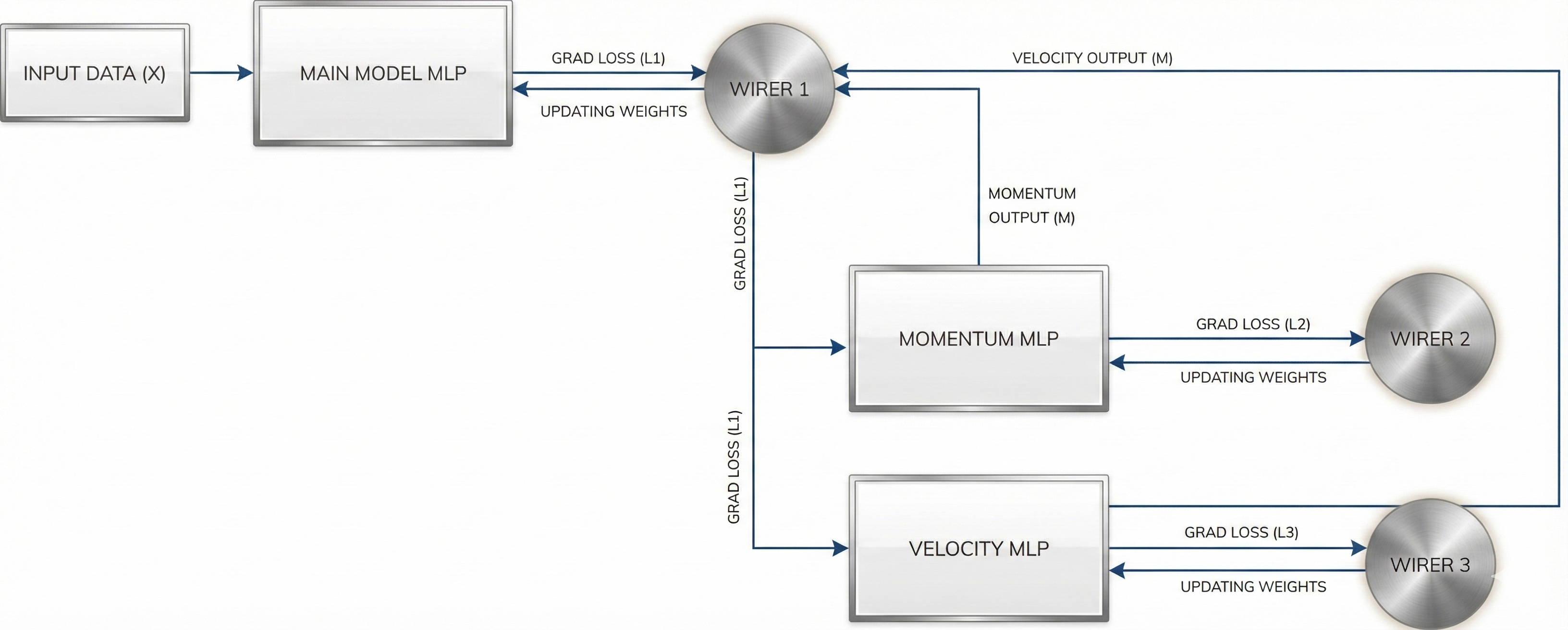
In Adam, we have another component, velocity ($v$), in addition to momentum. You can think of it as yet another memory model, but it would be at the same level as momentum (parallel learning), and our main Wirer 1 would then use both the values of momentum and velocity to make its updates.

Velocity, just like momentum, is a single-valued memory with no weights. We can convert it to have its own set of parameters as well, and the process could continue in a similar fashion.

6. Conclusion and Future Directions

What we discussed above is the simplest kind of Nested Learning, where the outer main model memory learns “how to map keys to values,” and the inner momentum and velocity memories learn “how to learn to map keys to values better.”

Therefore, using Adam for training any machine learning model represents a 2-layered memory paradigm of nested learning with three memory models.

This is the first part of my work to simplify and expand on the concept of Nested Learning. In the second part, I will discuss how we can actually calculate the $P$ vector, which we are using as the gold label to train our momentum MLP. I will explain the part of the paper concerning multiple frequencies and provide my insights on it before exploring new ideas in this direction.

Acknowledgments

This work would obviously not have been possible without the groundbreaking paper from Google Research. I extend my gratitude to the authors for their innovative contribution to the field.

References

[1] Ali Behrouz, Meisam Razaviyayn, Peiling Zhong, and Vahab Mirrokni. Nested Learning: The Illusion of Deep Learning Architectures. Google Research, USA, 2025.